Home | Raytracing Reference | Help
The degree of a product term such as x^2 * y^3 * z^4 is the sum of the exponents of the various variables appearing in the term. In this case, the degree of the term is (2 + 3 + 4) = 9.
The degree of a polynomial expression is the highest of the degrees of its terms. For example, the degree of
x^4 + x^2 + xy + y^2 + xy^2 + xy^4
is 5 (= 1 + 4 in the last term). An expression of degree n is referred to as an nth-degree expression. For example,
ax^2 + bx + c = 0
is a second degree equation.
Many objects cannot be modelled as surfaces. Examples are clouds and fog. These are described as density maps. A density map is a function that gives the (you guessed it!) density of an object at any point in space. The higher the density at a particular place, the more opaque/solid is the object at that place. Clouds, for example, would use some sort of fractal density map, with the bulk of the cloud of moderate density and opaque, and the little wispy things sticking out of low density and more "see-through". Fog uses a constant density map or one that decreases with height.
The main step in rendering a density map is to find how much light is reflected and how much is transmitted in a particular direction. This is done by integration techniques. We move in the given direction in small steps, adding the density of the current position to the total as we move along. If the total is large, the density map is more or less opaque in that direction; if it small, it is translucent.
Raytracers use a recursive algorithm for calculating the colour of a point. Now this recursion cannot continue for ever, but the computer isn't clever enough to understand that without being explicitly told to stop at some point. So we have the depth counter. Depth refers to how deep the ray tree extends, i.e., it is an index of the level of recursion. If the raytracer is told to stop at a trace depth of 2, then it follows the ray through two reflections and refractions and halts. Obviously, the higher the trace depth, the more realistic is the picture and the longer is the rendering time. But in most cases, after a few reflections/refractions, the intensity of the rays becomes so low that further intensity increments have very little effect on the total value. Trace depths of 5 usually produce fairly realistic pictures. With a depth of 0, raytracing degenerates to raycasting.
Note: the paragraph above describes depth in the sense most relevant to raytracing, i.e. that of trace depth. Depth can in fact be a counter of the level of recursion of any recursive process, such as octree subdivision and adaptive subdivision antialiasing.
A derivative is the fundamental concept of the branch of mathematics known as calculus. Simply put, a derivative describes the rate of change of a quantity -- e.g., velocity is the derivative of position because it measures the rate of change of position. Mathematically speaking, the derivative of the function f(x) with respect to x is calculated as
The derivative is written as f'(x) or dy/dx, where y = f(x). In a graph of the function f(x), the derivative at a point is the slope of the tangent to the graph at that point. Higher order derivatives describe the rate of change of functions that are derivatives themselves. For example, the derivative of f'(x) is called the second-order derivative of f(x) and is written as f''(x). Third and higher order derivatives are written as f'''(x), f''''(x) and so on. A better way is to write f'(x), f''(x) and f'''(x) as
Derivatives are indispensible in just about any branch of mathematical science known to man. In physics, derivatives help us study quantities that are rapidly changing. E.g., velocity and acceleration are the first and second order derivatives of the position function with respect to time; the emf induced in a closed conducting loop is given by the rate of change of the magnetic flux through it. In mathematics, useful data regarding the nature of a function can be obtained by studying its derivatives, apart from their simple geometrical use of calculating tangents. In a raytracer, derivatives have their principal uses in calculating the normal to a surface and computing the roots of an equation, especially if the Newton-Raphson method is used.
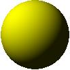
Most real surfaces are not perfect reflectors, they are rough and scatter light. In the Lambertian model, the strongest scattering takes place when the surface is perpendicular to the incident light, and a light-to-dark gradient is observed. Renderers model this effect by assigning each surface a "diffuse reflectivity coefficient" kD. The perceived intensity is calculated as kD(N.L), where N is the unit surface normal vector and L is the unit vector from the surface point to the light source. Lambertian intensity is independent of viewing direction. The perceived colour is calculated as (Lambertian intensity * surface colour * light colour).
There are other models of diffuse reflection, including those that have intensity peaks around the direction of ideal reflection. These produce shiny spots (Phong highlights) on the surface which do depend on the viewing direction.
A dimension of a system is a variable parameter. Any state in an n-dimensional system can be completely characterized by exactly (but not less than) n dimensions. A flat sheet is two dimensional, since it has two variable surface parameters of width and length. The world as we know it has three dimensions of space (3-D). Space-time is 4-dimensional, with the extra dimension of time. An ideal gas system is 3-dimensional, having the dimensions of pressure (P), volume (V) and temperature (T).